While searching for ways to create a thematic map of Switzerland, I came across the impressive website of Timo Grossenbacher. In his blog he describes the construction of a Swiss map using two well-known R packages: ggplot2 and sf.
The spatial structure of the map is based on geo-data of all Swiss municipalities. The Swiss Federal Statistical Office (FSO) makes this geo-data, i.e. shape or polygon data of the municipal boundaries, freely available. Each municipality can be identified by an id defined by the FSO. The id is crucial to join any data with individual municipalities. Whether population data, voting results, or even data about energy consumption, the id allows any data to be mapped to the municipality level.
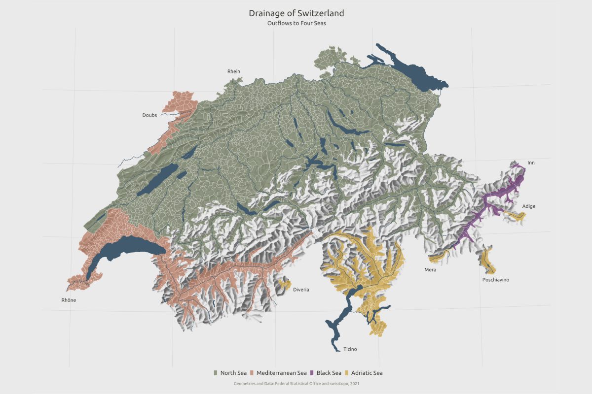
The topic of the following experiment is deliberately kept very simple: I want to depict into which seas the individual municipalities of Switzerland ultimately drain. Four destinations are available: the North Sea, the Mediterranean Sea, the Adriatic Sea and the Black Sea.
The Geo Data
Let’s have a look at the data. The current geo-shapes for the total of 2’172 Swiss municipalities in 2021 are available under this link. Download and extract the whole zip-file into a folder – named for instance /input – directly on the working directory of the R project (see the R script below).
If you take a closer look at the geo-file for the municipalities (again, the path and the name of this file can be seen in the following R script), you can see in it, besides the actual geo-shape data (i.e. the boundary polygons), for each of the listed municipalities, the id mentioned above as well as the corresponding municipality name.
Besides the municipality data, the download also provides geo-files for the rivers and lakes of Switzerland which we will use as well.
Somewhat special is the fact that the geo-file subtracts from the total area of each municipality those areas that are devoid of vegetation (e.g. glaciers, rocks, boulders, …) as well as those areas that are above 2’000 meters above sea level.
The omitted non-vegetation areas are left blank and are ultimately overlaid with a relief image in tif-format (see header image above). The relief image is originally from swisstopo. Unfortunately, I couldn’t discover the original link to it, so I’ve chosen an alternative URL for downloading this relief file named 02-relief-georef-clipped-resampled.tif.
The Theme Data
I manually created the assignment of the four drainage destinations to the individual Swiss municipalities. Starting point was the mentioned list of municipalities in the FSO geo-dataset. For each municipality identified by id and name I added the runoff destination manually and finally saved the list as a csv-file (named: themeData.csv). The following table shows selected examples of the theme file.
| id | name | outflow |
|---|---|---|
| … | ||
| 4941 | Märstetten | North Sea |
| 4946 | Weinfelden | North Sea |
| 4951 | Wigoltingen | North Sea |
| … | ||
| 5001 | Arbedo-Castione | Adriatic Sea |
| 5002 | Bellinzona | Adriatic Sea |
| 5003 | Cadenazzo | Adriatic Sea |
| … | ||
| 5497 | Pompaples | Mediterranean Sea |
| 5498 | La Sarraz | Mediterranean Sea |
| 5499 | Senarclens | Mediterranean Sea |
| … | ||
| 3746 | Zernez | Black Sea |
| 3752 | Samnaun | Black Sea |
| 3762 | Scuol | Black Sea |
The R code
Here now is the R script. I took large parts of the script from Timo Grossenbacher’s publication, but also simplified it a lot. We start by including the needed R packages and by reading the downloaded data from the mentioned /input folder. Note the join operation at the end of the following code snippet.
|
1 2 3 4 5 6 7 8 9 10 11 12 13 14 15 16 17 18 19 20 21 22 23 24 25 26 27 28 29 30 31 32 33 34 35 36 37 38 39 40 41 42 43 44 45 46 47 48 49 50 51 52 53 54 |
############################################################################################################### # Drawing a Swiss map with ggplot2 and sf using geodata at the municipality level # Exemplary theme: Drainage of Switzerland # Author: Albert Blarer # 2021-11-22 # Template: Timo Grossenbacher (e.g.: https://timogrossenbacher.ch/2019/04/bivariate-maps-with-ggplot2-and-sf/) ############################################################################################################### library(tidyverse) # ggplot2, dplyr, tidyr, readr, purrr, tibble library(magrittr) # pipes library(sf) # spatial data handling library(raster) # raster handling (needed for relief) # Read all geodata (source: FSO) # Municipalities municipality_geo <- read_sf("input/2021_GEOM_TK/GEOM_2021/01_INST/Vegetationsfl„che_vf/K4_polg20210101_vf/K4polg20210101vf_ch2007Poly.shp") head(municipality_geo,100) # just have a look at the first 10 rows of the data # Lakes and rivers lake1_geo <- read_sf("input/2021_GEOM_TK/GEOM_2021/00_TOPO/K4_seenyyyymmdd/k4seenyyyymmdd11_ch2007Poly.shp") # lakes- category 1 (i.e. > 500 ha) lake2_geo <- read_sf("input/2021_GEOM_TK/GEOM_2021/00_TOPO/K4_seenyyyymmdd/k4seenyyyymmdd22_ch2007Poly.shp") # lakes- category 2 (i.e. > 195-499 ha) # Compile the data into one table lake_geo <- rbind(lake1_geo,lake2_geo) head(lake_geo,10) river1_geo <- read_sf("input/2021_GEOM_TK/GEOM_2021/00_TOPO/K4_flusyyyymmdd/k4flusyyyymmdd11_ch2007.shp") river2_geo <- read_sf("input/2021_GEOM_TK/GEOM_2021/00_TOPO/K4_flusyyyymmdd/k4flusyyyymmdd22_ch2007.shp") river3_geo <- read_sf("input/2021_GEOM_TK/GEOM_2021/00_TOPO/K4_flusyyyymmdd/k4flusyyyymmdd33_ch2007.shp") river4_geo <- read_sf("input/2021_GEOM_TK/GEOM_2021/00_TOPO/K4_flusyyyymmdd/k4flusyyyymmdd44_ch2007.shp") river5_geo <- read_sf("input/2021_GEOM_TK/GEOM_2021/00_TOPO/K4_flusyyyymmdd/k4flusyyyymmdd55_ch2007.shp") # Compile the data into one table river_geo <- rbind(river1_geo,river2_geo,river3_geo,river4_geo,river5_geo) head(river_geo,10) # Raster of relief (original open source: swisstopo) relief <- raster("input/02-relief-georef-clipped-resampled.tif") relief_spdf <- as(relief, "SpatialPixelsDataFrame") # Relief is converted to a data frame relief <- as.data.frame(relief_spdf) %>% rename(value = `X02.relief.georef.clipped.resampled`) # Read the manually compiled thematic, i.e. outflow data themeData <- read_csv("input/themeData.csv") head(themeData,10) # Join municipality geodata with thematic data (first convert the join variables into the same data type ) themeData$id <- as.numeric(themeData$id) municipality_geo$id <- as.numeric(municipality_geo$id) municipality_geo %<>% left_join(themeData, by = c("id" = "id")) head(municipality_geo,10) |
After reading in the data, we define some global constants, e.g. for colors, fonts, etc..
|
1 2 3 4 5 6 7 8 9 10 11 12 13 |
# Define some constants default_background_color <- "#efefef" default_grid_color <- "#dbdbd9" default_municipality_border_color <- "#ffffff" default_water_color <- "#516d81" default_outflows <- c("Adriatic Sea", "Black Sea","Mediterranean Sea","North Sea") default_outflow_colors <- c("#d9b14c","#7e4080","#c78a6e","#818a6f") default_font_family <- "Ubuntu Regular" default_font_color <- "#4e4d47" default_caption_color <- "#939184" default_title <- "Drainage of Switzerland" default_subtitle <- "Outflows to Four Seas" default_caption <- paste0("Data & Geometries: Federal Statistical Office and swisstopo, 2021") |
Now we get to the actual map creation. The function theme_list() creates a list of basic theme attributes, such as grid lines, borders, background color, spacings, title and legend texts with position, font, etc..
|
1 2 3 4 5 6 7 8 9 10 11 12 13 14 15 16 17 18 19 20 21 22 23 24 25 26 27 28 29 30 31 32 33 34 35 36 37 38 39 40 41 42 43 44 45 46 47 48 49 50 51 52 |
# Define a map theme; returns a list theme_list <- function(...) { theme_minimal() + theme( # define the general font attributes text = element_text(family = default_font_family, color = default_font_color), # remove axes elements axis.line = element_blank(), axis.text.x = element_blank(), axis.text.y = element_blank(), axis.ticks = element_blank(), # add a subtle grid panel.grid.major = element_line(color = default_grid_color, size = 0.2), panel.grid.minor = element_blank(), # define background colors plot.background = element_rect(fill = default_background_color, color = NA), panel.background = element_rect(fill = default_background_color, color = NA), legend.background = element_rect(fill = default_background_color, color = NA), # borders and margins plot.margin = margin(t=.5, b=.5, l=.5, r=.5, unit="cm"), panel.border = element_blank(), panel.spacing = unit(c(.2,.2,.2,.2), "cm"), # legend and titles legend.position = "bottom", legend.margin=margin(t=-.3, b=.0, unit = "cm"), legend.box.margin=margin(t=.0, b=.4, unit = "cm"), legend.title = element_blank(), legend.key.size = unit(.4,"line"), legend.text = element_text(size = 10, hjust = .5, color = default_font_color), plot.title = element_text(size = 15, hjust = .5, color = default_font_color, margin = margin(b=0.1, t=0.1, unit = "cm"), debug = F), plot.subtitle = element_text(size = 10, hjust = 0.5, color = default_font_color, margin = margin(b=0.1, t=0.1, unit = "cm"), debug = F), # captions at the bottom of the graph plot.caption = element_text(size = 7, hjust = .5, margin = margin(t = 0, b = 0, unit = "cm"), color = default_caption_color), ... ) } |
The overlaying of the individual map layers is done as follows: First, we prepare the relief image and set it as background.
On top of that we put the municipality data with the respective boundaries and the (color) distinguishable variable outflow, which was joined to it via the municipality id and represents the different outflow destinations.
Finally, we embed the layers of lakes and rivers into the map, as well as the design of text elements.
|
1 2 3 4 5 6 7 8 9 10 11 12 13 14 15 16 17 18 19 20 21 22 23 24 25 26 27 28 29 30 31 32 33 34 35 36 37 38 39 40 41 42 43 44 45 46 47 48 49 50 51 52 53 54 55 56 57 58 59 60 61 62 63 64 65 66 67 68 69 70 71 72 73 74 75 76 77 78 79 80 81 82 83 84 85 86 87 88 89 90 91 92 93 94 95 96 97 98 99 100 101 102 103 104 105 106 107 108 109 110 111 112 113 114 115 116 117 118 119 120 121 122 123 124 125 126 |
############## # Plot the map ############## map <- ggplot( # Define the main data source (i.e. the joined data) data = municipality_geo ) + # First: draw the relief geom_raster( data = relief, inherit.aes = FALSE, aes( x = x, y = y, alpha = value ) ) + # Use the "alpha hack", as the "fill aesthetic" is already taken) scale_alpha(name = "", range = c(0.7, 0.0), guide = "none") + # suppress legend # Add main fill aesthetic geom_sf( mapping = aes( fill = outflow # the thematic data ), # Use thin white stroke for municipality borders color = default_municipality_border_color, size = 0.1 ) + # Set the legend text and order it scale_fill_manual(values = alpha(default_outflow_colors,0.7), labels = default_outflows, guide = guide_legend(reverse = TRUE)) + # Draw lakes in blue geom_sf( data = lake_geo, fill = default_water_color, color = default_water_color, size = 0.2 ) + # Draw rivers in blue geom_sf( data = river_geo, fill = default_water_color, color = default_water_color, size = 0.3 ) + # Add titles and caption labs(x = NULL, y = NULL, title = default_title, subtitle = default_subtitle, caption = default_caption) + # Add the theme theme_list() # Annotate the outflowing river names annotations <- tibble( label = c( "Doubs", "Rhône", "Rhein", "Inn", "Adige", "Poschiavino", "Mera", "Ticino", "Diveria" ), coord = c( "554050, 242000", # Doubs "493000, 102000", # Rhône "617000, 275000", # Rhein "834000, 206000", # Inn "830000, 173000", # Adige "810000, 120000", # Poschiavino "765000, 125000", # Mera "695000, 65000", # Ticino "657000, 110000" # Diveria ), just = c( "1,0", # Doubs "1,0", # Rhône "1,0", # Rhein "0,0", # Inn "0,0", # Adige "0.5,1", # Poschiavino "1,0", # Mera "0,0", # Ticino "0,0" # Diveria ) ) %>% separate(coord, into = c("x", "y")) %>% separate(just, into = c("hjust", "vjust"), sep = "\\,") annotations %>% pwalk(function(...) { # Collect all values in the row in a one-rowed data frame current <- tibble(...) # Convert all columns from x to vjust to numeric current %<>% mutate_at(vars(x:vjust), as.numeric) # Update the plot object with global assignment map <<- map + # For each annotation, add the label geom_text( data = current, aes( x = x, y = y, label = label, hjust = hjust, vjust = vjust ), # Set sfont tyles family = default_font_family, color = default_font_color, size = 3 ) }) # Finally show the map map |
The map is ready so far. In order to name the most important outflows, i.e. outflowing rivers of Switzerland and put them on the map, we use a simple annotation system. For example the Rhine (Rhein), which drains the largest area of Switzerland into the North Sea. Next to it the Doubs, which flows into the Rhône via Saône and finally drains into the Mediterranean. In the south and southeast of Switzerland, five border crossing rivers drain into the Adriatic Sea via the Po. And in the far east of Switzerland, the Inn flows eastwards and meets the Danube (Donau) in Passau, which finally drains into the Black Sea.
A respectable map, I think, which is just waiting to be fed with new data.